Explaining Missing Heritability Using Gaussian Process Regression (Reader's Digest)
Summary
The paper “Explaining Missing Heritability Using Gaussian Process Regression” by Sharp et al. tries to tackle the problem of missing heritability and the detection of higher-order interaction effects through Gaussian process regression, a technique widely used in the machine learning community. The authors obtained estimates of broad-sense heritability for a number of mice and yeast phenotypes using a RBF kernel that models higher-order interactions, and found these estimates significantly larger than the narrow-sense heritability of these phenotypes. The authors also deteced several loci displaying interaction effects.
Background
Heritability
In genetics, phenotypes are modeled by the following equation \[ y_i = f(x_i) + u_i + \epsilon_i, \] where \( y_i \) is the phenotype measurement of the i-th individual, \( x_i \) the genotype vector, \( u_i \) a random effect term that captures relatedness among individuals, and \( \epsilon_i \) the environmental noise. Here, \( f(\cdot) \) is a function that maps the genotype vector into a real number. Under this model, heritability is defined as the proportion of variance in \( y_i \) that is due to variation of \( f(x_i) \), \[ \text{heritability} = { {\text{Var}[f(x)]} \over {\text{Var}[y]} } \]
Different flavors of heritability exist based on the complexity of the \( f(\cdot) \) function and the input that goes into \( f(\cdot) \). In general geneticists work with four types of heritability, as listed below.
-
Broad-sense heritability (\( H^2 \)): Broad-sense heritability is the amount of variance in phenotypes that is due to all genetic variations including both additive and epistatic effects. For \( H^2 \), the function \( f(\cdot) \) can be any function that incoporates any order of interactions between genetic variations. This is the most general definition of heritability.
-
Narrow-sense heritability (\( h^2 \)): Narrow-sense heritability is the amount of variance in phenotypes that is due to all additive genetic effects. For \( h^2 \), the function \( f(\cdot) \) is a linear function that takes in first-order terms.
-
SNP heritability ( \( h^2_g \) ): SNP heritability is the amount of variance in phenotypes that is due to additive genetic effects of a given set of SNPs. For \( h^2_g \), the function \( f(\cdot) \) is a linear function that takes in a fixed set of SNPs.
-
GWAS heritability ( \( h^2_{GWAS} \) ): GWAS heritability is the amount of variance in phenotypes that is due to additive genetic effects of GWAS hits. For \( h^2_{GWAS} \), the function \( f(\cdot) \) is a linear function that takes in GWAS hits only.
Based on the definition of the four flavors of heritability, it follows that \( H^2 > h^2 \ge h^2_g \ge h^2_{GWAS} \). The missing heritability problem often refers to the gap between \( h^2_{GWAS} \) and the narrow- / broad- sense heritability.
Gaussian Process Regression
Parametric regression problems often involve a function (\( f(\cdot) \)), governed by a set of parameters (\( \theta \)), that maps each input \( X \) with a response. For example, in Poisson regression (\( Y \sim Pois(\lambda = g(X^T\beta)) \)), the distribution of the response variable is characterized by the mean parameter \( \lambda \) and the density function of Poisson. \[ { {\lambda^k \exp(-\lambda)} \over {k!} } \]
Gaussian Process Regression is different from parametric regression in that one does not assume any parametric form for the function \( f(\cdot) \). Instead, a Gaussian Process prior assumes that the function values of \( f(\cdot) \), \( \mathbf{f} \), for a number of inputs, \( X \), follow a multivariate normal distribution, \[ \mathbf{f} \sim N(\mathbf{0}, \mathbf{K}), \] where \( \mathbf{K} = (\mathbf{K})_{ij} = \mathbf{k}(x_i, x_j) \) is the kernel matrix, measuring the similarity between samples, that contraints the possible space of \( f(\cdot) \). Because the only constraint on the kernel function \( \mathbf{k}(\cdot, \cdot) \) is that the covariance matrix \( \mathbf{K} \) is positive definite, this enables Gaussian Process Regression to model a broad range of functions.
The following is a list of kernel functions that are widely used (credit to Wikipedia),
- Linear kernel: \( \mathbf{k}(x_i, x_j) = x_i^Tx_j \)
- Polynomial kernel: \( \mathbf{k}(x_i, x_j) = (x_i^Tx_j + r)^n \text{ for } r > 0 \)
- RBF kernel: \( \mathbf{k}(x_i, x_j) = \exp \left( - { {||x_i - x_j||^2} \over {2\sigma^2} } \right)\)
Applying Gaussian Process Regression to Heritability Estimation
The Kernel Function
Specifying the kernel function is a fundamental step of Gaussian Process Regression. An appropriate kernel allows one to model interaction of any order among genetic variations. In the Sharp et al. paper, the authors proposed a generalized version of the RBF kernel to measure similarity between two individuals, \( x_i \) and \( x_j \), acorss the genotypes of \( P \) SNPs, \[ \mathbf{k}(x_i, x_j) = \theta_0 \exp \left( -\sum_{p=1}^P { {(x_{ip}-x_{jp})^2} \over {2 \tau_p} } \right), \] where \( \theta_0 \) is a parameter that governs the overall similarity between \( x_i \) and \( x_j \), \( \tau_p \) the contribution of SNP \( p \) to the variations of the phenotype – a large \( \tau_p \) suggests that SNP \( p \) contributes little to the variation of the phenotype, and a small \( \tau_p \) implies significant contribution. By examining the magnitude of the hyperparameters \( \tau_p \), one can infer whether a genetic loci contribute significantly to the trait.
Sparsity-Inducing Priors
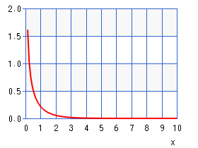
Overfit may occur when the number of parameters to estimate is larger than the amount of data one has. To avoid overfitting and improve parsimony of the model, the authors imposed a Gamma prior over the inverse of \( \tau_p \), \( \tau_p^{-1} \). The Gamma prior has density function \[ p(\tau_p^{-1}) = { {(\alpha_x / \mu_x)^{\alpha_x} } \over {\Gamma(\alpha_x)} } (\tau_p^{-1})^{(\alpha_x-1)} \exp \left( - { {\alpha_x\tau_p^{-1} } \over {\mu_x} } \right). \] Setting \( \alpha_x = 0.5 \) removes any mode in the density function, resulting in a monotonically decreasing function with a heavy tail concentrated around 0 (see figure below), enforcing most of \( \tau_p^{-1} \) to be close to zero.
Posterior Distribution of the Parameters
Gaussian Process prior allows one to analytically perform integration over the space of \( f(\cdot) \), resulting in a posterior for the parameters \( \theta = (\tau_1, \cdots, \tau_p, \theta_0) \), \[ p(\theta | X, y, \Phi) \propto N(y | 0, \mathbf{K} + \tau_e^{-1} I) p(\theta | \Phi), \] where \( p(\theta | \Phi) \) incoporates the sparsity-inducing priors. The integration step effectively averages over all possible \( f(\cdot) \), discarding the need to estimate each instance of \( f(\cdot) \) separately. This step also increases power to detect loci that contribute to phenotypes.
There is no analytical solution to the posterior mode or mean of \( \theta \). However, sampling based approach (e.g. MCMC) can be used to start from a starting point and lead to the posteior mode. In the Sharp et al. paper, a Hybrid Monte Carlo that models a particle’s trajectory was used to make inference over \( \theta \).
Estimating Broad-Sense Heritability
Once the parameters \( \theta = (\tau_1, \cdots, \tau_p, \theta_0) \) are estimated, one can use these estimates to quantify broad-sense heritability from the Gaussian Regression model. The basic idea is as follows:
- For each sample in the training data, one first predits its phenotype using the estimated parameters.
- The variance of the predicted phenotype can be found analytically using the conditional distribution of multivariate normal.
- The ratio between the sum of each individual’s variance and the phenotype variance gives the broad-sense heritability.